MV-7013: Inverted Pendulum Control Using MotionSolve with Compose Subroutines
In this tutorial, you will learn how to use MotionView, MotionSolve, and Compose to design a control system that stabilizes an inverted pendulum.
The goal of this tutorial is to design a regulator using the pole placement method. The inverted pendulum MDL model file is supplied.
- Check the stability of the open loop system.
- Export linearized system matrices A, B, C, and D using MotionSolve linear analysis.
- Design a controller using Compose.
- Implement a controller in MotionView.
- Check the stability of a closed loop system using MotionSolve linear analysis.
- Add disturbance forces to the model and run simulation using MotionSolve.
The image below shows the classic inverted pendulum on a slider. The system has two degrees of freedom leading to four state variables. The vertically upright position of the pendulum is unstable. The goal is to design a regulator to stabilize this configuration.
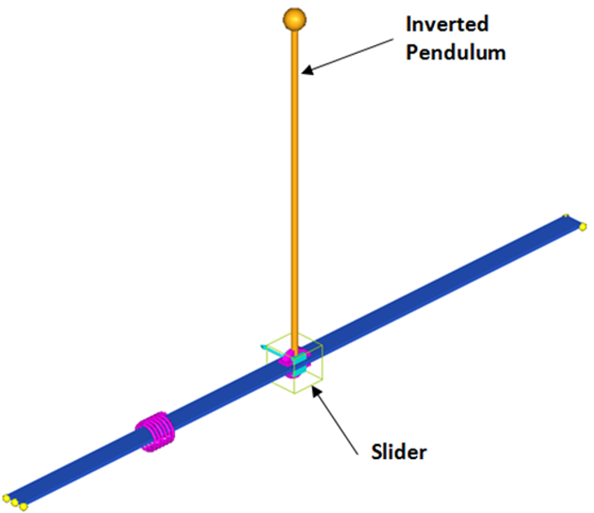
Figure 1. Inverted Pendulum Model
To achieve the goal, find a full-state feedback control law. The control input is a force applied to the slider along the global X-axis. Plant output is the pendulum angle of rotation about the global Y-axis.
Start by loading the file inv_pendu.mdl, located in [installation_directory]\tutorials\hwdesktop\mv_hv_hg\mbd_modeling\motionsolve, into MotionView and save it to your working directory. Upon examination of the model topology, notice that everything needed for this exercise is included in the model. However, depending on which task you are performing, it may be necessary to activate or deactivate certain entities.
References: Feedback Control of Dynamic Systems, G. G. Franklin, J. D. Powell, and A. Emami-Naeini, Third Edition, Addison Wesley.
Determine the Stability of the Open Loop Model
Compute the eigenvalues to determine the stability of the inverted pendulum.
-
From General Actions toolbar, click Run,
 .
.
-
From the Results Browser, select individual modes.
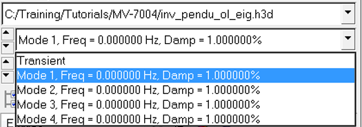
Figure 2. -
Click Start/Pause Animation,
 , to visualize the mode shape.
Obtain a Linearized Model
Usually, the first step in a control system design is to obtain a linearized model of the system in the state space form:
ẋ = Ax+Bu
y = Cx+Du
where A, B, C, and D are the state matrices, x is the state vector, u is the input vector, and y is the output vector. The A, B, C, and D matrices depend on the states chosen (by the solver), inputs, and outputs. You only need to define the inputs and outputs.
-
Click Run, .
-
Specify the output filename as
inv_pendu_state_matrices.xml.

Figure 3. Linear Tab in the Simulation Settings Dialog for Specifying the Compose Matrix Files Output -
From the Main tab, click Run.
A new file is created with the base name inv_pendu_state_matrices.oml.The states chosen by the MotionSolve solver are:
- Angular displacement about the global-Y axis.
- Translation displacement along the global X-axis.
- Angular velocity about the global-Y axis.
- Translation velocity along the global X-axis of the pendulum body center of mass marker.
Note: MotionSolve writes the selected states into the log file if Write debug info is selected under Output Options.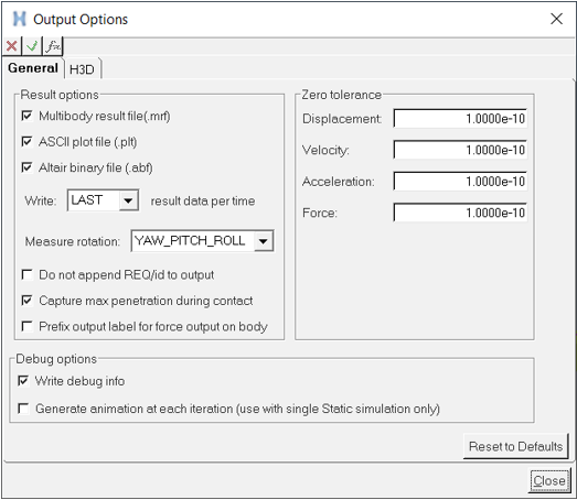
Figure 4. General Tab in Output Options Dialog for Specifying the Write debug info.
Design a Control System in Compose
A detailed discussion of control system design is beyond the scope of this tutorial. However, the steps to design a regulator using pole placement[1] to stabilize the inverted pendulum are described briefly. For details, refer to the standard controls text and the Compose documentation.
- Employ a full-state feedback control law u = − k ∗ x, where u is the control input, k is the gain vector, and x is the state vector.
- Assuming the necessary pole locations are stored in vector P, use the pole placement method to compute k.
- Load the state space matrices into the Compose workspace by loading/running the script inv_pendu_state_matrices.oml.
- For poles P at 3 Hz, type the following into the command window:
p = 2*pi*3 * [ -1 -1 -1 -1 ] ; k = acker( A , B , p ) - The Compose
acker function yields to the following processing and result:
k = [Matrix] 1 x 4
-15020.22034 -12.86975 -2806.23453 -2.74083
Implement the Control Force in MotionView
The control force is u = − k ∗ x. The model contains a solver variable called Control Force Variable - CL. Replace the Force Entity with a user-defined Compose script using GFOSUB. GFOSUB accesses the states of the system via m_sysfnc.
Write the Compose Script
-
Close the function with an end command.
Below is an example of the complete function, with your script resembling the following example:
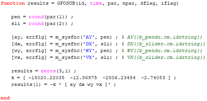
Figure 5.
Implement the Compose Script
-
From the User-Defined tab, edit the Force value with the
Expression Builder to include the pendulum and slider marker
idstring.
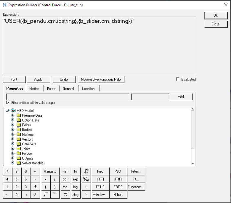
Figure 6. -
Use
 to select GFOSUB.oml from your
<working directory>.
to select GFOSUB.oml from your
<working directory>.
-
Verify Function name is set to GFOSUB.
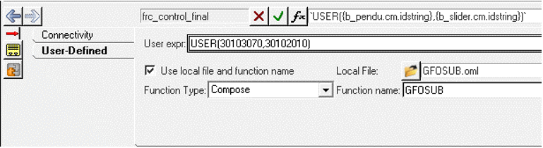
Figure 7.
Check the Stability of a Closed Loop System
-
Specify the output file as inv_pendu_cl_eig.xml and click
Run, .
The eigenvalues are shown below.
NUMBER NATURAL_FREQ(HZ) DAMPING_RATIO REAL(HZ) IMAG_FREQ(HZ) 1 2.681249E+00 1.000000E+00 -2.681249E+00 0.000000E+00 2 3.380362E+00 1.000000E+00 -3.380362E+00 0.000000E+00 3 2.989457E+00 9.933140E-01 -2.969470E+00 3.451144E-01 4 2.989457E+00 9.933140E-01 -2.969470E+00 -3.451144E-01 They all have negative real parts, hence the system is stabilized. Note that the negative real parts are close to the necessary poles ( 3 Hz ).
Add Disturbance Force and Run a Transient Simulation
-
From the toolbar, click Run, .
-
The plots of disturbance force, control force, slider x displacement, and
pendulum angular displacement are shown below.
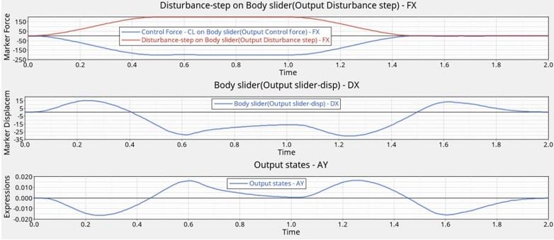
Figure 8. Plots of Disturbance and Control Forces as well as Slider Translational and Pendulum Angular Displacements