In this tutorial, you will learn to:
| • | Run a simple normal modes analysis. The default solver used is OptiStuct. |
This exercise uses the Full_Motion_TV_Mount_Partly_Open.hm file, which can be found in the hm.zip file. Copy the file(s) from this directory to your working directory.
Normal modes analysis is a method to calculate the normal modes or the modes at which an object resonates at its natural frequencies. It can also be called Eigenvalue analysis or Eigenvalue extraction. If a thorough normal modes analysis is not carried out, a structure can fail catastrophically due to resonance. Loads applied at specific points can cause a structure to resonate and cyclic loading at such points can lead to failure. If a constraint is not defined in a loadstep a free-free boundary condition will be assumed and the first six modes found will be the rigid body modes.
|
| 1. | Launch HyperMesh. The User Profiles dialog opens. |
| 2. | Select BasicFEA from the Application drop-down and click OK or click Preferences > User Profiles to open the dialog. |
| Note: | You can also launch BasicFEA from the Start menu by clicking All Programs > Altair <version > BasicFEA. |
|
|
| 1. | Copy the model provided for linear static analysis into a directory on your computer. |
| 2. | Right-click anywhere in the BasicFEA browser. This opens a context menu that contains several relevant functions. |
| 3. | Click Open to display a dialog that allows you to load the model. |
| 4. | Browse to the directory on your computer where the model is stored and load the model by selecting it and clicking Open. The model used for this tutorial is Full_Motion_TV_Mount_Partly_Open.hm. This model does not contain any other information except geometry information and units metadata. BasicFEA organizes and creates properties and materials upon import. |
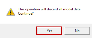
| Note: | When you load the model into BasicFEA all existing model data is deleted and replaced. |
|
| Note: | Pressing CTRL on the keyboard while clicking the model allows you to zoom in and out. |
|
|
| 1. | After the model is loaded, the wireframe geometry of the model is displayed. To view the model better and to get a feel for the way it looks after fabrication, click the  icon in the BasicFEA toolbar. icon in the BasicFEA toolbar. |
| 2. | Right-click Mode: Geometry in the BasicFEA browser and select Mesh to view the default mesh on the model. BasicFEA generates a default mesh for the model without the need for you to do anything. |
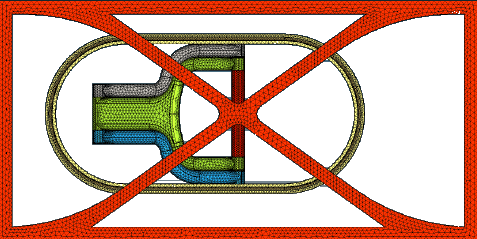
Meshed model
| 3. | The mode is changed back to Geometry for the rest of the analysis setup. |
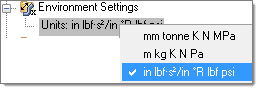
| 4. | The units of the model are set up by default, but you can change them by right-clicking Units in the BasicFEA browser. For this exercise the English FPS system is used (in Ibf-s^2/in *R Ibf psi). |
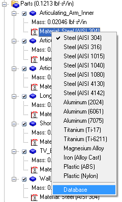
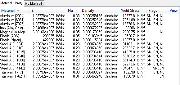
| 5. | Materials are assigned by default for each part. Right-clicking a part and selecting Material provides a list that contains the commonly used materials. Clicking Database opens a Material Database dialog with the complete database of all available materials. |
| 6. | Click the My Materials tab and the plus icon to add a new user defined material to the database. |
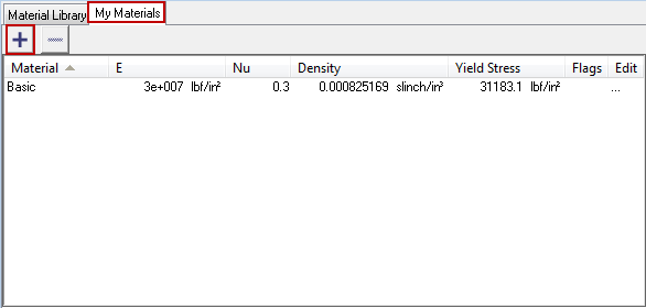
| 7. | Name the new material Basic and change the Young's Modulus (E) to 3.0 e 07 and the Poisson's ratio (Nu) to 0.3. |
| 8. | Close the Material Database dialog. |
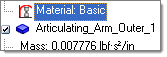
| 9. | After the new material is added, right-click Material underneath any of the parts and select Basic from the list of materials. The name of the material now shows. |
| 10. | The dimensions of the model can be checked by clicking the  icon in the BasicFEA toolbar. This step is optional. icon in the BasicFEA toolbar. This step is optional. |
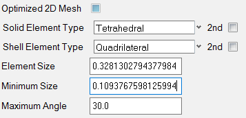
| 11. | If the default model settings are not satisfactory you can change them by right-clicking a part and selecting Mesh Settings. This opens the Mesh Settings dialog. This step is optional. |
|
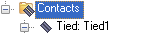
Since the model consists of different parts, they have to be connected before analysis. The simplest form of connection is a tied contact between touching parts.
| 1. | Right-click Contacts in the BasicFEA browser and select Create > Auto-contact. Auto contact will search the model for touching parts and create a tied contact between each of them. |
|
| 1. | As you have seen in the previous step, the right-click context menu is used to create a new normal modes loadstep. Right-click Loadsteps and select Create > Normal Modes Loadstep. After the loadstep is added the default values for the analysis are accepted. |
| 2. | Right-click in the BasicFEA browser and select Save as to save the model before analysis. Select any location you prefer to save the model and save it as a HyperMesh (.hm) file. |
| Note: | The surfaces for which you want to apply constraints or loads turn white in color as you click on them. This makes it easier for you to distinguish them from the other surfaces. |
|
|