Indoor Intelligent Ray Tracing
The indoor intelligent ray-tracing method accelerates ray optical models and reduces the computation time to that of empirical models. This method combines the advantages of both ray optical models and neglects their disadvantages. It is based on a single preprocessing of the building data base.
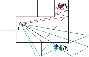
Figure 1. Principle of ray optical models.
In a first step, the walls of the buildings will be divided into tiles and the edges into horizontal and vertical segments, see Figure 2. After this discretization of the database the visibility relationships of the different elements are determined and stored in a file. For this process all elements are represented by their centers. This leads to a simplification of the problem of ray path finding (possible interaction points are only the centers of the tiles and segments). The visibility relations between each tile (segment) and all other tiles (segments) are computed in the pre-processing, because they are independent of the transmitter and receiver locations.
For the decision about the visibility relation, the line of sight criterion between the centers of the tiles (or segments) is evaluated. If there is line of sight between the centers, the rays from the center of the first tile to the corners of the second tile are determined and the projection of the angles of the rays on the first and second tile are stored together with the visibility relation. A similar computation for the visibility relations between tiles and segments and between segments and other segments is done and also stored in the file of the pre-processing.
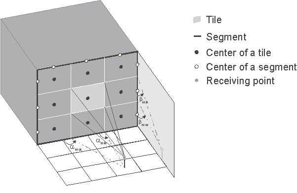
Figure 2. Subdivision of the building database into small elements.
The angles of the projection are important, because they define a range of possible reflection (or diffraction) angles for the illuminated tile (or segment). The angle also continues on the neighboring tile, so a very accurate prediction of the rays is possible even if the tiles or segments are large (up to 50 or 100 meters for urban data bases). A further improvement is possible if the grid of the prediction points is also used in the pre-processing, because the prediction plane can be subdivided into tiles and the visibility relations between the tiles of the prediction grid and the tiles (and segments) of the walls represent the last part of the ray in the direction to the receiver.
If the receiver visibility relations are determined in the pre-processing, the only remaining visibility relations to be computed in the prediction are the ones from the transmitter to the tiles (of walls and prediction grid) and segments.
An example for the visibility relations between a tile and a receiving point is shown in Figure 2. For the calculation of the angles the connecting straight lines between the receiving point and the four edges of the tile are considered.
By projecting these four lines into the xy-plane and additionally into a plane perpendicular with respect to the inspected wall, four angles are determined which give an adequate description of this visibility relation.
Propagation Paths
This deterministic model allows an accurate rigorous 3D Ray Tracing prediction, because many interactions can be taken into account. The selection of propagation paths is similar to the method for the standard ray-tracing (SRT). Therefore each transmission through a wall, each reflection at a wall and each diffraction at an edge counts as an interaction. Due to a pre-processing of the database the IRT model has a short computation time.
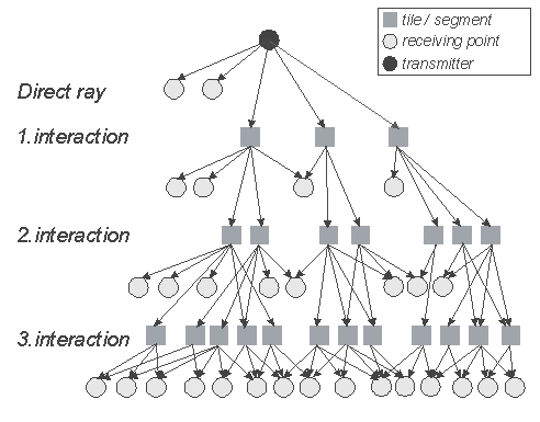
Figure 3. Determination of ray paths by searching in a tree structure.
The result of the pre-processing of the building data base is a tree structure containing tiles, segments and receiving points of the prediction area, see Figure 3. In this tree every branch symbolizes a visibility relationship between two elements. For the prediction only the tiles, segments and receiving points, which are visible from the base station have to be determined. Additionally, the angles of incidence for the visible tiles and segments have to be calculated. The relations in the first layer of the tree must be computed in the prediction, all other relations are determined in the pre-processing and can be read from a file.
The ray search is stopped, if a receiving point or a given maximum number of interactions is reached. Finally the field strength is summed up at all potential receiving points.
Settings

Figure 4. The Parameter: Intelligent Ray Tracing (IRT) dialog.
- Propagation Paths - Number of Interactions
-
The Settings dialog allows to specify how many interactions should be considered for the determination of ray paths between transmitter and receiver including maximum number of reflections, diffractions and scattering.
Example: If Max Reflections AND Diffractions AND Scattering is 2 and if Max. Reflections is 2 and Max. Diffractions is 2, the rays with a total of 2 interactions have either 2 reflections or 2 diffractions or one reflection and one diffraction. Rays with more than two interactions are not considered in this case.
If Max Reflections AND Diffractions AND Scattering is 4, Max. Reflections is 2 and Max. Diffractions is 2, we will compute the following rays- 0 interaction: 0 R and 0 D
- 1 interaction: 1 R and 0 D (R), 0 R and 1 D (D)
- 2 interactions: 2 R and 0 D (R - R), 1 R and 1 D (R - D and D - R), 0 R and 2 D (D - D)
- 3 interactions: 3 R and 0 D (R - R - R), 2 R and 1 D (R - R - D and R - D - R and D - R - R), 1 R and 2 D (R - D - D and D - R - D and D - D - R), 0 R and 3 D (D - D - D)
- ...
- ...
The higher the value for Max Reflections AND Diffractions AND Scattering, the longer the computation time.
Diffuse scattering in indoor scenarios can play an important role, especially for determining the actual temporal and angular dispersion of the radio channel. The IRT model for indoor scenarios have been extended to consider the scattering on building walls and other objects. For this purpose the scattering can be activated in the model settings (where also the number of reflections and diffractions are defined). As the scattering increases the overall number of rays significantly, there is a limitation of one scattering per ray. The single scattering is considered as separate ray and also in combination with other interactions (transmission, reflection and diffraction).
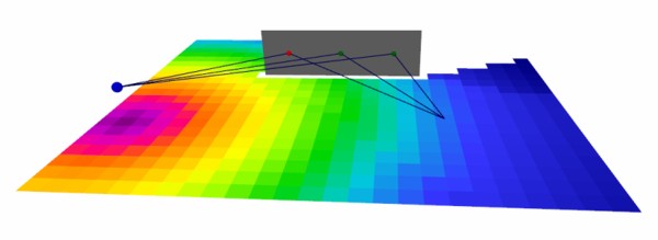
Figure 5. Diffuse scattering.
Furthermore the scattering properties of the corresponding materials need to be defined (in WallMan and ProMan). Both the empirical and the deterministic (physical) interaction models are supported. In the empirical interaction model the scattering loss defines the additional loss (for a ray 30° out of the reflection direction). The scattering loss is added to the reflection loss. The defined scattering loss is applied if the angle difference between reflected and scattered ray is 30°. In case of 0° no additional scattering loss is applied. Generally the scattering loss is increasing with increasing angular difference. In the deterministic model the polarimetric scattering matrix S_vv, S_vh, S_hv, S_hh is defined and considered for the field strength computation. For the scattering in the IRT model the tiles as defined in the WallMan pre-processing are considered. The scattered contribution is weighted with the size of the scattering area (tile) with a reference size of 100 sqm. Accordingly the resulting scattered power from the whole object is for large distances independent of the tile size. For small distances there is an impact due to the modified scattering angles which depend on the tile size
- Propagation Paths - Selection of Paths
-
- Limitation of number of paths per pixel with the following options
-
- maximum path loss of rays
- maximum number of paths
- dynamic range of paths
- Consideration of Rays for Computation of Angular Spread and Mean
-
During computation of delay or angular spread and mean, the contribution of each propagation path to the delay or angular spread/mean is considered. Each path contributes a signal level to the spread. This level can be either considered as power (in dBm or Watt) or as field strength (in dBµV/m or in µV/m). Power values include the gain of the Rx antenna and depend on the frequency, whereas field strength values do not depend on the frequency. The values can be considered either in logarithmic scale (dBm or dBµV/m) or in linear scale (mW or µV/m).
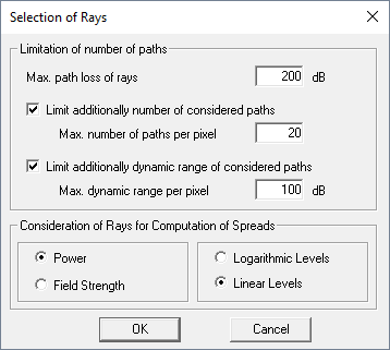
Figure 6. Selection of rays dialog.
- Propagation Paths - Direct ray
- The direct ray can be computed always, despite the number of transmissions specified in the first section.
- Computation of Interaction Losses of the Rays
- For the computation of the rays, not only the free space loss has to be considered but also the loss due to the transmissions, reflections and (multiple) diffraction. This is either done using a physical deterministic model or using an empirical model similar to the method for the standard ray tracing (SRT).
- Path Loss Exponent for Ray-Optical Models
- Exponent for distance dependent path loss.
- Superposition of Contributions
- Superposition of contributions of different rays can be done either incoherent (without consideration of the phases) or coherent (with consideration of the phases).