SS-T: 4070 Random Response Analysis
Create random response analysis in SimSolid.
Purpose
SimSolid performs meshless structural
analysis that works on full featured parts and assemblies, is tolerant of
geometric imperfections, and runs in seconds to minutes. In this tutorial,
you will do the following:
- Create dynamic random analysis for a walkway assembly with base excitation load.
Model Description
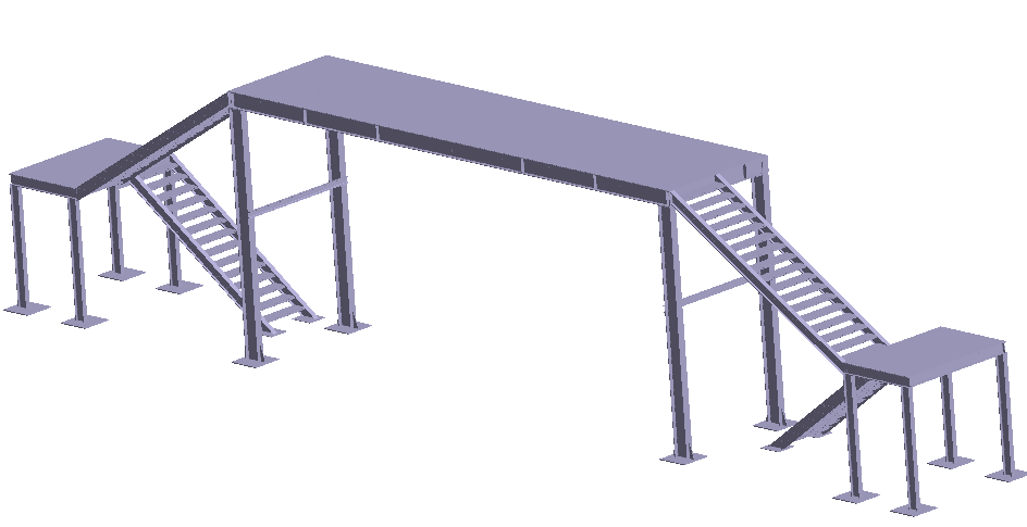
Figure 1.
The following files are needed for this tutorial:
- Random.ssp
- PSD_Function.csv
The project file has the following specifications:
- Material is set to Steel for all parts.
- Regular connections with 3mm gap and penetration tolerance.
Open Project
Open the SimSolid project file.
-
Click the
 (Open Project) icon.
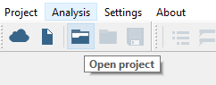
Figure 2.
Create Modal Analysis
-
On the main window toolbar, click the
 (Modal analysis) icon.
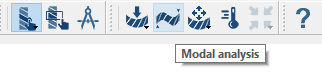
Figure 3.
Create Immovable Support
Create immovable supports on select faces in the model.
-
In the Analysis Workbench, click
 (Immovable support).
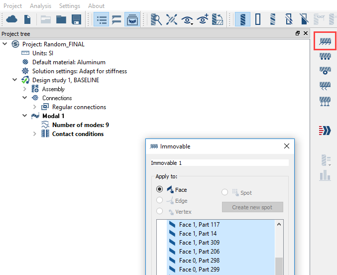
Figure 4. -
In the modeling window, select the two faces shown in
orange in Figure 5.
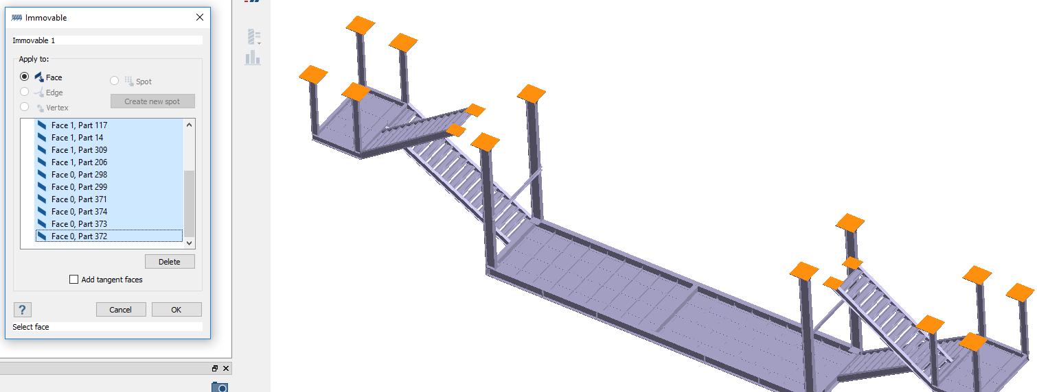
Figure 5.
Run Analysis
Solve the analysis.
- In the Project Tree, open the Analysis Workbench.
-
Click
 (Solve).
Review Results
Plot displacement magnitude contour and review the modes.
-
On the Analysis Workbench, select
 > Displacement Magnitude.
The Legend widow will open and display the contour plot. The Frequency (Hz) window will open and list the modes.
> Displacement Magnitude.
The Legend widow will open and display the contour plot. The Frequency (Hz) window will open and list the modes.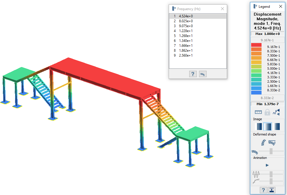 Figure 6.
Create Random Response Analysis
Use modal results to create random response analysis.
-
On the main window toolbar, select
 > Random response.
The Dynamic random response setup dialog will open and automatically link to the Modal analysis results.
> Random response.
The Dynamic random response setup dialog will open and automatically link to the Modal analysis results.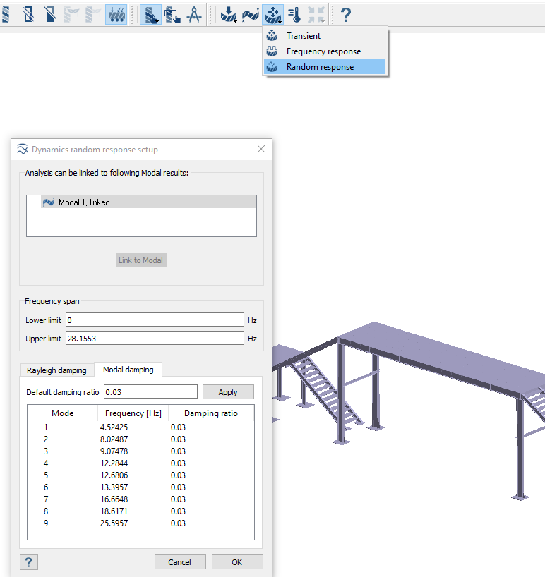
Figure 7.
Create PSD Functions
Define power spectral density (PSD) vs frequency response.
-
On the workbench toolbar, click the
 (Power Spectral Density function) icon.
-
In the dialog, click the Import CSV button.
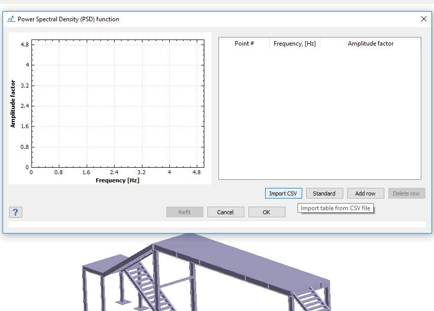
Figure 8. -
In the File explorer, browse to the PSD_Function.csv file
and click Open.
The function will be plotted in the XY graph in the dialog.
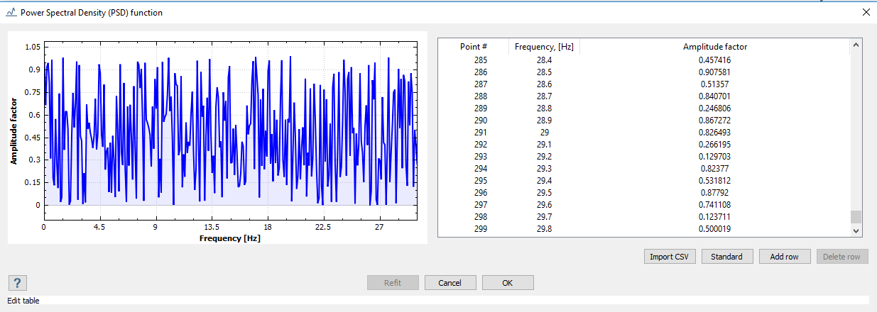
Figure 9.
Define Loads
Define base excitation load.
-
On the Assembly workbench toolbar, click the
 (Base excitation) icon.
-
For direction, enter 1 for X, Y, and Z.
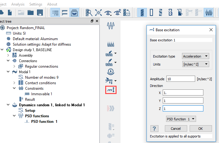
Figure 10.
Run Analysis
Solve the analysis.
- In the Project Tree, open the Analysis Workbench.
-
Click (Solve).
Review Results
Plot displacement magnitude contour and review the modes.
-
On the Analysis Workbench, select > Displacement Magnitude.
The Legend widow will open and display the contour plot. The Dynamics random response window will open. You can use the slider to animate frequencies.
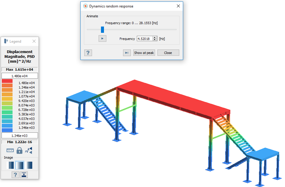
Figure 11.
Plot Response Curve
Plot response vs frequency for a picked location and obtain partial response.
-
On the workbench toolbar, click the
 (Pick info) icon.
-
In the modeling window, select a point on the model as
shown in Figure 12.
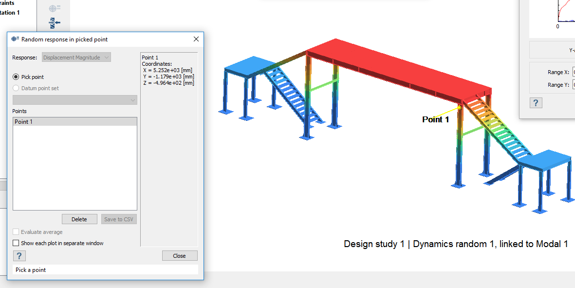
Figure 12.The response for the point will be plotted in the XY graph in the dialog. You can use the scroll wheel to zoom in, the left mouse button to pan, or the Refit button to reset the graph.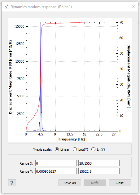
Figure 13. -
Obtain Partial Response.
-
In the dialog, pick a point on the curve to show the Modes
contributions into response table.
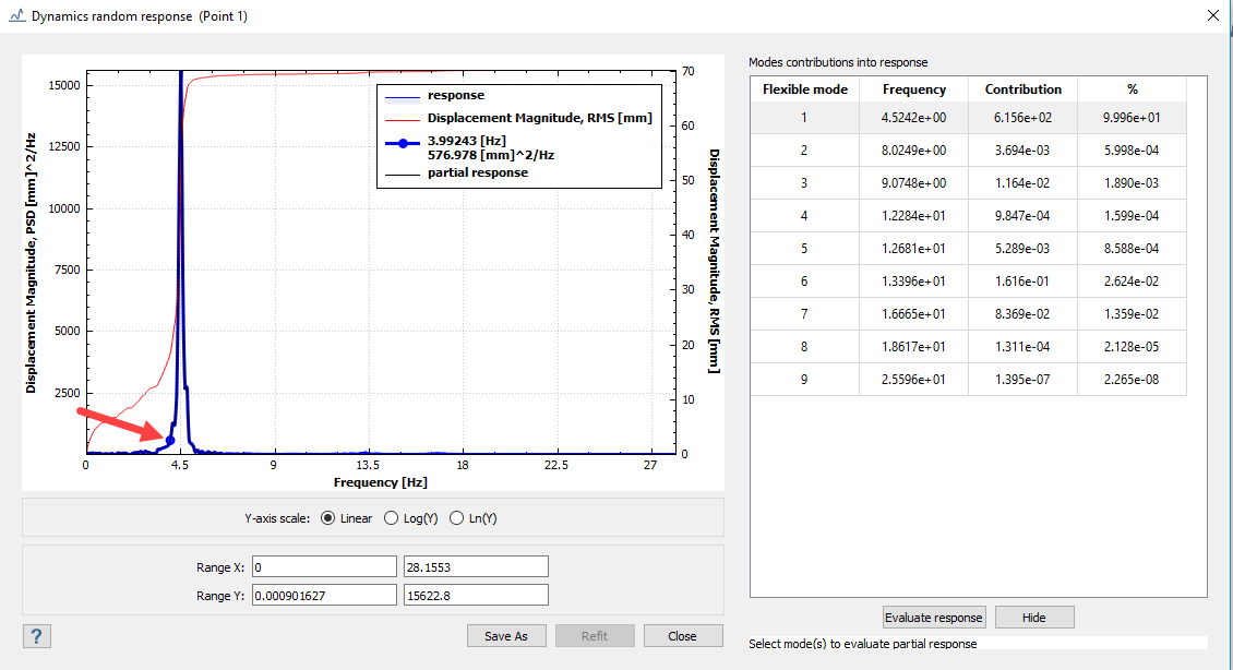
Figure 14.
The plot in the dialog will update to show the partial response. -
In the dialog, pick a point on the curve to show the Modes
contributions into response table.