Example 9: 14x14 Coaxial Feed Array with Binomial Algorithm

This case explains how to use the binomial algorithms to calculates the pointing parameters in a bidimensional coaxial feed array.

Step 1 Create a new MoM Project.

Open newFASANT and select File - New option.

Figure 1. New Project panel

Select MOM option on the previous figure and start to configure the project.

Step 2 Set the simulation parameters as shown.

Select Simulation - Parameters option, set the parameters and save it.

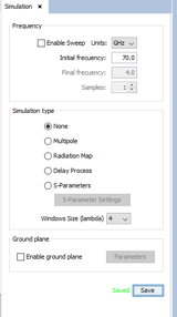
Figure 2. Simulation panel

Step 3 Create the array

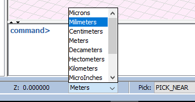
First, select 'milimeters' on units list on the bar at the bottom of the main window.

The first element is created using Source - Coaxial Feed - Add Feed Point.

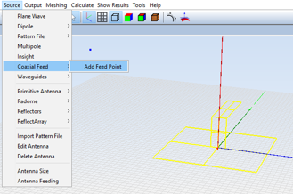
Figure 3. Add feed point

Select the surfaces and click on Add.

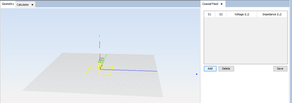
Figure 4. Coaxial Feed panel

Then save the feed point.

Use the array command and enter the characteristics of the array.

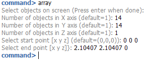
Figure 5. Array parameters

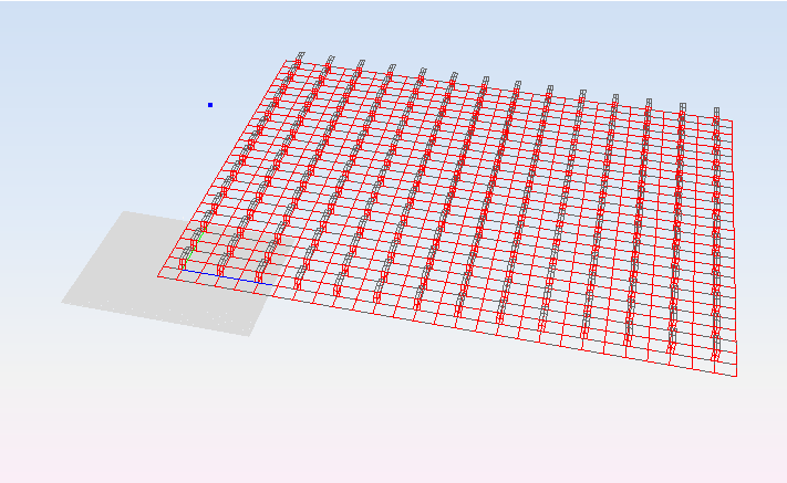
Figure 6. Array view

Step 4 Feed the array

To set the feeding of the array select Source - Antenna Feeding and the following panel will open.

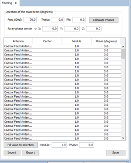
Figure 7. Antenna Feeding panel

This is the default setting. To use the binomial algorithm click on Tools - User Function and select the corresponding function (which can be downloaded). NOTE To use the bidimensional binomial function it is needed to download both the bidimensional and the unidimensional functions.

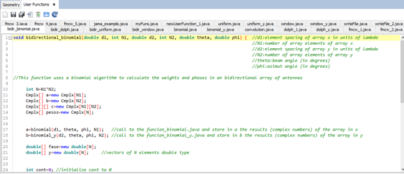
Figure 8. Bidimensional Binomial function

A path has been selected by default so the files will be created on the mydatafiles folder in the newFASANT directory.

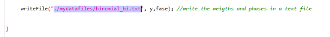
Figure 9. Bidimensional Binomial function

The next step is generating the text file. To do so click on Tools - Calculator and write the call to the function.

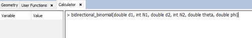
Figure 10. Calculator panel

The parameters to set are:

· d1: element spacing of the array in the x-axis in units of lambda

· N1: number of array elements of the array in the x-axis

· d2: element spacing of the array in the y-axis in units of lambda

· N2: number of array elements of the array in the y-axis

· theta: beam angle, in degrees

· phi: azimuth angle, in degrees

In this case, set the parameters as shown. Angles of theta=30º and phi=0º are selected as an example.

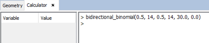
Figure 11. Calculator panel

A spacing of 0.5 in units of lambdas is selected because is equivalent to a spacing of 2.104 millimeters at 70 GHz.

The text file will be automatically generated in the mydatafiles folder.

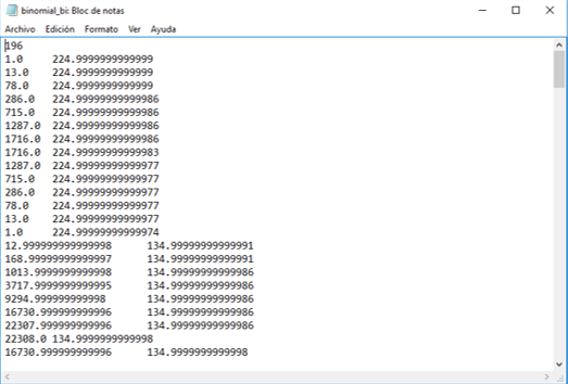
Figure 12. Results file

Now, apply these results to the array created before by clicking on Source - Antenna Feeding.

The panel shown before will appear. To use the weights and phases calculated with the binomial algorithm, click on Import.

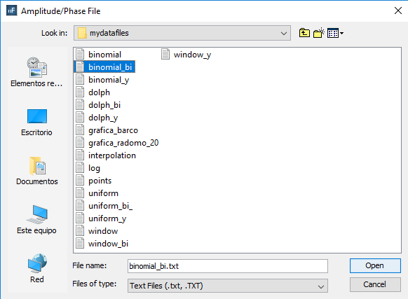
Figure 13. Amplitude/Phase File panel

Select the corresponding file and save the feeding.

Step 5 Solver parameters

Select Solver - Advanced Options and set the parameters as shown.

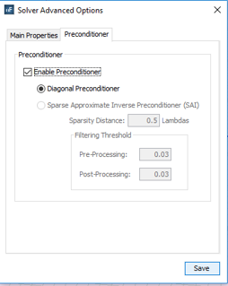
Figure 14. Solver Advanced Options panel

Step 6 Meshing the geometry model.

Select Mesh - Create Mesh to open the meshing configuration panel and then set the parameters as show the next figure.

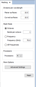
Figure 15. Meshing panel

Step 7 Execute the simulation.

Select Calculate - Execute option to open simulation panel.

Figure 16. Calculate panel

Step 8 Show Results

The radiation cuts can be visualized by clicking on Show Results - Radiation Pattern - View Cuts.

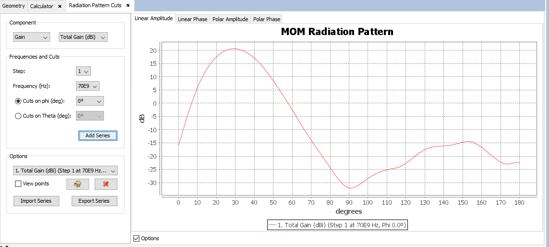
Figure 17. Radiation Pattern Cuts

The radiation pattern can be visualized by clicking on Show Results - Radiation Pattern - View 3D Pattern.

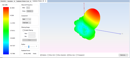
Figure 18. Radiation Pattern 3D